x = 5
y = "Hello, Julia!"
Julia Syntax Essentials and Variable Scoping
Julia is fundamentally an imperative programming language, where the flow of execution is defined by sequences of commands or statements that change the program’s state. Core features include:
- Assignment statements to store values in variables.
- Control flows for decision-making and iteration.
- Arithmetic operations for calculations.
While imperative programming emphasizes how a task is accomplished (e.g., through loops, conditionals, and assignments), declarative programming focuses on what the result should be, leaving the “how” to the language or framework. Julia is versatile and can incorporate elements of declarative programming, such as high-level operations on collections and functional programming paradigms, but its foundation is firmly rooted in imperative concepts.
Tip
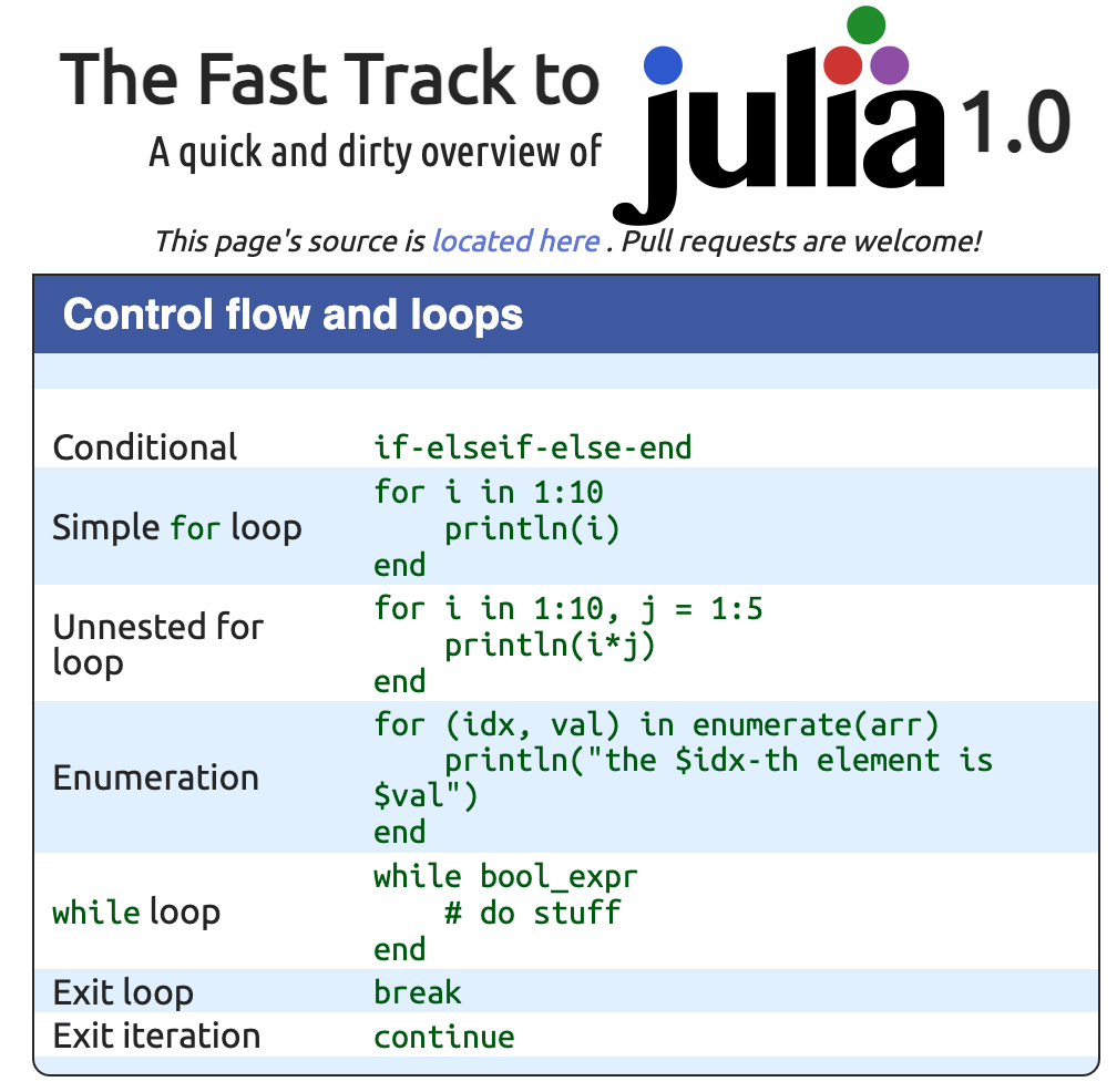
In this page, we present the fundamentals of Julia syntax. If you want a cheatsheet, click on the image below.
Basics
Assignment
In Julia, variables are assigned using the = operator:
Julia is dynamically typed, which means variables do not require explicit type declarations. Types are inferred based on the assigned value.
typeof(x)Int64typeof(y)StringVariables act as labels pointing to values and can be reassigned without restrictions on type. This dynamic behavior is a hallmark of imperative languages.
Unicode Characters
Julia supports Unicode characters, enhancing code readability, especially for mathematical and scientific computations:
α = 10
β = α + 5
println("β = $β")
β = 15Unicode symbols can be entered using \name followed by Tab (e.g., \alpha → α). A complete list of Unicode characters is available in the Julia Unicode documentation.
Printing Output
For debugging or displaying results, Julia provides the println function:
println("Hello, Julia!")  # Prints: Hello, Julia!
println("The value of α is ", α)
Hello, Julia!
The value of α is 10Additionally, the @show macro prints both variable names and values:
x = 42
@show x   # Prints: x = 42
x = 42You can also use @show with multiple variables or expressions:
a = 10
b = 20
@show a + b  # Prints: a + b = 30
@show a, b   # Prints: a = 10, b = 20
a + b = 30
(a, b) = (10, 20)Comparison Operations
Julia includes standard comparison operators for equality and order:
| Operator | Purpose | Example | Result |
|---|---|---|---|
== |
Equality check | 5 == 5 |
true |
!= or ≠ |
Inequality check | 5 != 3 |
true |
<, <= |
Less than, or equal | 5 < 10 |
true |
=== |
Object (type and value) identity check | 5 === 5.0 |
false |
Examples:
5 == 5     # true
5 != 3     # true
5 ≠ 3      # true (using Unicode)
5 < 10     # true
10 >= 10   # true
"Julia" === "Julia"  # true (identical strings)
5 === 5.0  # false (different types: Int vs. Float)
julia> 5 == 5 = true
julia> 5 != 3 = true
julia> 5 ≠ 3 = true
julia> 5 < 10 = true
julia> 10 >= 10 = true
julia> "Julia" === "Julia" = true
julia> 5 === 5.0 = falseJulia’s comparison operators return Bool values (true or false). Using these operators effectively is essential for control flow and logical expressions.
In Julia, the === operator checks object identity, meaning it determines if two references point to the exact same memory location or the same instance. This is a stricter comparison than ==, which only checks if two values are equivalent in terms of their contents, not if they are the same instance.
Here’s a breakdown of === in Julia:
Singletons:
===is often used for checking singleton objects likenothing,true,false, and other immutable types that Julia reuses rather than copying. For instance,nothing === nothingwill returntrue, and similarly,true === truewill returntrue.Immutable Types: For immutable types like
Int,Float64, etc.,===and==usually give the same result since identical values are often the same instance.Performance:
===is generally faster than==because it doesn’t need to do a value comparison, just a memory location check. This is particularly useful when checking if a value is a specific singleton (e.g.,x === nothing).
a = 1
b = 1
a === b  # true, since 1 is an immutable integer, they are identical instances

x = [1, 2]
y = x
x === y  # true, because x and y refer to the same object in memory

x == [1, 2]   # true, because the contents are the same
x === [1, 2]  # false, because they are different instances in memory
julia> a = 1
julia> b = 1
julia> a === b = true
julia> x = [1, 2]
julia> y = [1, 2]
julia> x === y = true
julia> x == [1, 2] = true
julia> x === [1, 2] = falseIn summary, === is especially useful for checking identity rather than equality, often applied to singletons or cases where knowing the exact instance matters, as it allows for efficient and clear comparisons.
Control Flows and Logical Operators
Control flow in Julia is managed through conditional statements and loops. Logical operators allow for conditions to be combined or negated.
Conditional Statements
Julia supports if, elseif, and else for conditional checks:
x = 10

if x > 5
    println("x is greater than 5")
elseif x == 5
    println("x is equal to 5")
else
    println("x is less than 5")
end
x is greater than 5In Julia, blocks for if, elseif, and else are closed with end. Indentation is not required by syntax but is recommended for readability.
Tip
You can follow the Blue Style conventions for Julia code. If you want to format your code you can use the package JuliaFormatter.jl.
Ternary Operator
For simple conditional assignments, Julia has a ternary operator ? ::
y = (x > 5) ? "Greater" : "Not greater"
println(y) # Outputs "Greater" if x > 5, otherwise "Not greater"GreaterLogical Operators
Julia includes standard logical operators, that combine or negate conditions:
| Operator | Purpose | Example | Result |
|---|---|---|---|
&& |
Logical AND | true && false |
false |
|| |
Logical OR | true || false |
true |
! |
Logical NOT | !true |
false |
a = true
b = false

a && b
a || b
!a
julia> a = true
julia> b = false
julia> a && b = false
julia> a || b = true
julia> !a = falseLoops
Julia provides for and while loops for iterative tasks.
For Loop: The for loop iterates over a range or collection:
for i in 1:5
    println(i)
end
1
2
3
4
5This loop prints numbers from 1 to 5. The range 1:5 uses Julia’s : operator to create a sequence.
Note
The for construct can loop on any iterable object. Visit the documentation for details.
While Loop: The while loop executes as long as a condition is true:
count = 1

while count <= 5
    println(count)
    count += 1
end
1
2
3
4
5This loop will print numbers from 1 to 5 by incrementing count each time.
Breaking and Continuing
Julia also has break and continue for loop control.
breakexits the loop completely.continueskips the current iteration and moves to the next one.
for i in 1:5
    if i == 3
        continue  # Skips the number 3
    end
    println(i)
end
1
2
4
5for i in 1:5
if i == 4
break # Exits the loop when i is 4
end
println(i)
end1
2
3These control flows and logical operators allow for flexibility in executing conditional logic and repeated operations in Julia.
Arithmetics
Julia supports a variety of arithmetic operations that can be performed on numeric types. Below are some of the most commonly used operations:
Basic Arithmetic Operations
You can perform basic arithmetic operations using standard operators:
- Addition:
+ - Subtraction:
- - Multiplication:
* - Division:
/(returns a floating-point result) and//(returns a rational number)
a = 10
b = 3

sum = a + b
difference = a - b
product = a * b
quotient = a / b
rational = a // b
julia> a = 10
julia> b = 3
julia> sum = 13
julia> difference = 7
julia> product = 30
julia> quotient = 3.3333333333333335
julia> rational = 10//3Modulo Operation
The modulo operator % returns the remainder of a division operation. It is useful for determining if a number is even or odd, or for wrapping around values.
modulus_result = a % b # remainder of 10 divided by 31Exponentiation
You can perform exponentiation using the ^ operator.
a^2 # 10 squared100Using Arithmetic in Control Flow
You can combine arithmetic operations with control flow statements. For example, you can use the modulo operation to check if a number is even or odd:
if a % 2 == 0
    println("$a is even")
else
    println("$a is odd")
end
10 is evenSummary of Arithmetic Operations
| Operation | Symbol | Example | Result |
|---|---|---|---|
| Addition | + |
5 + 3 |
8 |
| Subtraction | - |
5 - 3 |
2 |
| Multiplication | * |
5 * 3 |
15 |
| Division | / |
5 / 2 |
2.5 |
| Modulo | % |
5 % 2 |
1 |
| Exponentiation | ^ |
2 ^ 3 |
8 |
These arithmetic operations can be combined and nested to perform complex calculations as needed.
Functions
Julia offers flexible ways to define functions, with options for positional arguments, keyword arguments, optional arguments with default values, and variable-length arguments. Let’s explore each of these in detail.
Defining Functions
Functions in Julia can be defined using either the function keyword or the assignment syntax.
# Using the `function` keyword
function add(a, b)
    return a + b
end

# Using assignment syntax
multiply(a, b) = a * b

add(2, 3)
multiply(2, 3)
julia> add(2, 3) = 5
julia> multiply(2, 3) = 6Positional and Keyword Arguments
In Julia, functions can take both positional arguments and keyword arguments.
Positional Arguments: These are listed first in the parameter list and must be provided in the correct order when the function is called. Positional arguments can have default values, but it’s not required.
Keyword Arguments: Keyword arguments are specified after a semicolon (
;) in the parameter list. These arguments must be provided by name when calling the function. Like positional arguments, keyword arguments can have default values, but they don’t have to.
function greet(name; punctuation = "!")
    return "Hello, " * name * punctuation
end

println(greet("Alice"))
println(greet("Alice", punctuation = "?"))
Hello, Alice!
Hello, Alice?In this example, punctuation is a keyword argument with a default value of "!". You could also define a keyword argument without a default value if needed.
Variable Number of Arguments
Julia functions can accept an arbitrary number of arguments using the splatting operator .... These arguments are gathered into a tuple.
function sum_all(args...)
    total = 0
    for x in args
        total += x
    end
    return total
end

sum_all(1, 2, 3, 4)
julia> sum_all(1, 2, 3, 4) = 10Default Values for Optional Arguments
In Julia, you can assign default values to both positional and keyword arguments. When the function is called without specifying a value for an argument with a default, the default value is used.
function power(base, exponent=2)
    return base ^ exponent
end

power(3)      # Outputs: 9 (since exponent defaults to 2)
power(3, 3)   # Outputs: 27
julia> power(3) = 9
julia> power(3, 3) = 27Multiple Optional Positional Arguments
When a function has multiple optional positional arguments, Julia will use the default values for any arguments not provided, allowing flexible combinations.
function calculate(a=1, b=2, c=3)
    return a + b * c
end

calculate()        # Outputs: 7  (1 + 2 * 3)
calculate(5)       # Outputs: 11 (5 + 2 * 3)
calculate(5, 4)    # Outputs: 17 (5 + 4 * 3)
calculate(5, 4, 1) # Outputs: 9  (5 + 4 * 1)
julia> calculate() = 7
julia> calculate(5) = 11
julia> calculate(5, 4) = 17
julia> calculate(5, 4, 1) = 9Here’s how the argument combinations work:
calculate()uses all default values:a=1,b=2,c=3.calculate(5)overridesa, leavingbandcas defaults.calculate(5, 4)overridesaandb, leavingcas the default.calculate(5, 4, 1)overrides all arguments.
This flexibility makes it easy to call functions with varying levels of detail without explicitly specifying each parameter.
Tip
If a function has many optional arguments, consider using keyword arguments to improve readability and avoid confusion about the order of arguments.
Mutation and the Bang ! Convention
In Julia, functions that modify or mutate their arguments typically end with a !, following the “bang” convention. This is not enforced by the language but is a widely followed convention in Julia to indicate mutation.
function add_one!(array)
    for i in eachindex(array)
        array[i] += 1
    end
end

arr = [1, 2, 3]
add_one!(arr)
arr  # Outputs: [2, 3, 4]
julia> arr = [1, 2, 3]
julia> add_one!(arr) = nothing
julia> arr = [2, 3, 4]In this example, add_one! modifies the elements of the array arr. By convention, the ! at the end of the function name indicates that the function mutates its input.
Broadcasting
Julia supports broadcasting, a powerful feature that applies a function element-wise to arrays or other collections. Broadcasting is denoted by a . placed before the function call or operator.
# Define a simple function
function square(x)
    return x^2
end

# Apply the function to a vector using broadcasting
vec = [1, 2, 3, 4]
squared_vec = square.(vec)

println("Original vector: ", vec)
println("Squared vector: ", squared_vec)
Original vector: [1, 2, 3, 4]
Squared vector: [1, 4, 9, 16]In this example:
- The function
square(x)is applied to each element ofvecusing the.operator. - Broadcasting works seamlessly with both built-in and user-defined functions, making it easy to perform element-wise operations on arrays of any shape.
Return Values
In Julia, functions automatically return the last evaluated expression. However, you can use the return keyword to explicitly specify the output if needed.
function multiply(a, b)
    a * b  # Returns the result of a * b
end
Scoping and Closure
In Julia, scoping rules determine the visibility and lifetime of variables. Understanding scope and closures is essential for writing efficient and error-free code.
Variable Scope
Scope in Julia refers to the region of code where a variable is accessible. There are two primary scopes: global and local.
- Global Scope: Variables defined at the top level of a module or script are in the global scope and can be accessed from anywhere in that file. However, modifying global variables from within functions is generally discouraged.
global_var = 10

function access_global()
    return global_var
end

access_global()  # Outputs: 10
julia> access_global() = 10- Local Scope: Variables defined within a function or a block (e.g., loops or conditionals) have local scope and cannot be accessed outside of that block.
function local_scope_example()
    local_var = 5
    return local_var
end

local_scope_example()
julia> local_scope_example() = 5If you try to access local_var outside the function, you will get an error because it is not defined in the global scope.
local_var # This would cause an error, as local_var is not accessible hereLoadError: UndefVarError: `local_var` not defined in `Main`
Suggestion: check for spelling errors or missing imports.
UndefVarError: `local_var` not defined in `Main`
Suggestion: check for spelling errors or missing imports.Scope of Variables in for Loops
In Julia, a for loop does create a new local scope for its loop variable when inside a function or another local scope. This means that a variable used as the loop variable will not overwrite an existing global variable with the same name in that context.
Here’s an example:
i = 10  # Define a global variable `i`

for i = 1:3
    println(i)  # Prints 1, 2, and 3
end

println("Outside loop: i = ", i)  # Outputs: 10
1
2
3
Outside loop: i = 10In this case, the initial value of i (10) is not affected by the loop because the for loop has its own local scope for i. After the loop completes, the global variable i retains its original value (10), demonstrating that the for loop did not alter it.
However, if this code were inside a function, i would be entirely scoped within that function’s local environment, meaning any loop variables would only affect other variables within the function itself.
Nested Scopes
Julia allows for nested functions, which can access variables in their enclosing scopes. This is known as lexical scoping.
function outer_function(x)
    y = 2
    function inner_function(z)
        return x + y + z
    end
    return inner_function
end

closure = outer_function(3)
closure(4)  # Outputs: 9 (3 + 2 + 4)
julia> closure(4) = 9In this example, inner_function forms a closure over the variables x and y, retaining access to them even after outer_function has finished executing.
Closures
A closure is a function that captures variables from its surrounding lexical scope, allowing the function to use these variables even after the scope where they were defined has ended. Closures are especially useful for creating customized functions or “function factories.”
Example: Using a Global Variable vs. Capturing a Variable in a Closure
To illustrate the difference between referencing a global variable and capturing a variable in a closure, let’s first create a function that uses a global variable:
factor = 2

function multiply_by_global(x)
    return x * factor
end

multiply_by_global(5)  # Outputs: 10

# Update the global variable `factor`
factor = 3
multiply_by_global(5)  # Outputs: 15 (factor is now 3)
julia> factor = 2
julia> function multiply_by_global(x)
return x * factor
end
julia> multiply_by_global(5) = 10
julia> factor = 3
julia> multiply_by_global(5) = 15In this example, multiply_by_global uses the global variable factor, so whenever factor is updated, the result of calling multiply_by_global changes.
Example: Capturing a Variable in a Closure
Now, let’s use a closure to capture the factor variable inside a function. Here, the captured value of factor remains fixed at the time the closure was created, regardless of changes to the variable afterward.
function make_multiplier(factor)
    return (x) -> x * factor  # Returns a closure that captures `factor`
end

double = make_multiplier(2)   # `factor` is captured as 2 in this closure
triple = make_multiplier(3)   # `factor` is captured as 3 in this closure

double(5)  # Outputs: 10
triple(5)  # Outputs: 15

# Even if we change `factor` globally, it doesn't affect the closure
factor = 4
double(5)  # Still outputs: 10
triple(5)  # Still outputs: 15
julia> function make_multiplier(factor)
return (x->begin
x * factor
end)
end
julia> double = make_multiplier(2)
julia> triple = make_multiplier(3)
julia> double(5) = 10
julia> triple(5) = 15
julia> factor = 4
julia> double(5) = 10
julia> triple(5) = 15In this example, make_multiplier returns a function that captures the factor variable when the closure is created. This means that double will always multiply by 2, and triple will always multiply by 3, regardless of any subsequent changes to factor.
Summary
Using closures in Julia allows you to “lock in” the values of variables from an outer scope at the time of the closure’s creation. This differs from referencing global variables directly, where any changes to the variable are reflected immediately. Closures are particularly useful for creating function factories or callbacks that need to retain specific values independently of changes in the global scope.
Understanding scope is crucial for performance in Julia. Defining variables within a local scope, such as inside functions, can lead to more efficient code execution. Global variables can lead to performance penalties due to type instability.
In summary, scoping rules in Julia allow for clear management of variable accessibility and lifespan, while closures enable powerful programming patterns by capturing the context in which they are created. Understanding these concepts is key to writing effective Julia code.
Exercices
Exercise 1: Temperature Converter
Write a function convert_temperature that takes a temperature value and a keyword argument unit that can either be "C" for Celsius or "F" for Fahrenheit. The function should convert the temperature to the other unit and return the converted value. Use a conditional statement to determine the conversion formula:
If the unit is
"C", convert to Fahrenheit using the formula: F = C \times \frac{9}{5} + 32If the unit is
"F", convert to Celsius using the formula: C = (F - 32) \times \frac{5}{9}
Example Output:
println(convert_temperature(100, unit="C"))  # Outputs: 212.0
println(convert_temperature(32, unit="F")) # Outputs: 0.0Exercise 2: Factorial Function with Closure
Create a function make_factorial that returns a closure. This closure should compute the factorial of a number. The closure should capture a variable that keeps track of the number of times it has been called. When the closure is called, it should return the factorial of the number and the call count.
Example Output:
factorial_closure = make_factorial()
result, count = factorial_closure(5)
println(result)  # Outputs: 120
result, count = factorial_closure(3)
println(result)  # Outputs: 6
println("Function called ", count, " times") # Outputs: 2 timesExercise 3: Filter Even Numbers
Write a function filter_even that takes an array of integers as input and returns a new array containing only the even numbers from the input array. Use a loop and a conditional statement to check each number.
Additionally, implement a helper function is_even that checks if a number is even. Use the filter_even function to filter an array of numbers, and print the result.
Example Output:
numbers = [1, 2, 3, 4, 5, 6, 7, 8, 9, 10]
even_numbers = filter_even(numbers)
println(even_numbers) # Outputs: [2, 4, 6, 8, 10]Exercise Instructions
- For each exercise, implement the required functions in a new Julia script or interactive session.
- Test your functions with different inputs to ensure they work as expected.
- Comment on your code to explain the logic behind each part, especially where you utilize control flow and scope.
Comments
Comments are written with the
#symbol. Julia also supports multiline comments with#=and=#: